
我正在尝试实现卡尔曼滤波器。我只知道位置。测量值在某些时间步丢失。这就是我定义矩阵的方式:
过程噪声矩阵
Q=np.diag([0.001,0.001])
测量噪声矩阵
R = np.diag([10, 10])
协方差矩阵
P = np.diag([0.001, 0.001])
观察矩阵
H = np.array([[1.0, 0.0], [0.0, 1.0]])
过渡矩阵
F = np.array([[1, 0], [0, 1]])
州
x = np.array([pos[0], [pos[1]])
我不知道这是否正确。例如,如果我在t=0处看到目标,而在t=1时没有看到目标,我将如何预测它的位置。我不知道速度。这些矩阵定义正确吗?
您需要扩展模型并为速度添加状态(如果需要,还可以为加速度添加状态)。过滤器将根据位置估计新的状态,并使用它们来预测位置,即使您没有位置测量。
你的矩阵看起来像这样:
过程噪声矩阵
Q = np.diag([0.001, 0.001, 0.1, 0.1, 0.1, 0.1]) #enter correct numbers for vel and acc
测量噪声矩阵保持不变
协方差矩阵
P = np.diag([0.001, 0.001, 0.1, 0.1, 0.1, 0.1]) #enter correct numbers for vel and acc
观察矩阵
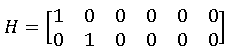
H = np.array([[1.0, 0.0, 0.0, 0.0, 0.0, 0.0], [0.0, 1.0, 0.0, 0.0, 0.0, 0.0]])
过渡矩阵
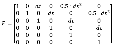
F = np.array([[1, 0, dt,  0, 0.5*dt**2,         0],
              [0, 1,  0, dt,         0, 0.5*dt**2],
              [0, 0,  1,  0,        dt,         0],
              [0, 0,  0,  1,         0,        dt],
              [0, 0,  0,  0,         1,         0],
              [0, 0,  0,  0,         0,         1]])
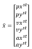
状态
看看我以前的帖子,有一个非常相似的问题。在这种情况下,只有加速度的测量和过滤器估计的位置和速度。
在原始加速度数据上使用PyKalman计算位置
在下面的帖子中,人们还必须预测位置。该模型仅由两个位置和两个速度组成。你可以在那里的python代码中找到矩阵。
具有可变时间步长的卡尔曼滤波器
更新
这是我的 matlab 示例,向您展示仅从位置测量中对速度和加速度的状态估计:
function [] = main()
    [t, accX, velX, posX, accY, velY, posY, t_sens, posX_sens, posY_sens, posX_var, posY_var] = generate_signals();

    n = numel(t_sens);

    % state matrix
    X = zeros(6,1);

    % covariance matrix
    P = diag([0.001, 0.001,10, 10, 2, 2]);

    % system noise
    Q = diag([50, 50, 5, 5, 3, 0.4]);

    dt = t_sens(2) - t_sens(1);

    % transition matrix
    F = [1, 0, dt,  0, 0.5*dt^2,        0;
         0, 1,  0, dt,        0, 0.5*dt^2;
         0, 0,  1,  0,       dt,        0;
         0, 0,  0,  1,        0,       dt;
         0, 0,  0,  0,        1,        0;
         0, 0,  0,  0,        0,        1];

    % observation matrix
    H = [1 0 0 0 0 0;
         0 1 0 0 0 0];

    % measurement noise
    R = diag([posX_var, posY_var]);

    % kalman filter output through the whole time
    X_arr = zeros(n, 6);

    % fusion
    for i = 1:n
        y = [posX_sens(i); posY_sens(i)];

        if (i == 1)
            [X] = init_kalman(X, y); % initialize the state using the 1st sensor
        else
            if (i >= 40 && i <= 58) % missing measurements between 40 ans 58 sec
                [X, P] = prediction(X, P, Q, F);
            else
                [X, P] = prediction(X, P, Q, F);
                [X, P] = update(X, P, y, R, H);
            end
        end

        X_arr(i, :) = X;
    end

    figure;
    subplot(3,1,1);
    plot(t, posX, 'LineWidth', 2);
    hold on;
    plot(t_sens, posX_sens, '.', 'MarkerSize', 18);
    plot(t_sens, X_arr(:, 1), 'k.', 'MarkerSize', 14);
    hold off;
    grid on;
    title('PositionX');
    legend('Ground Truth', 'Sensor', 'Estimation');

    subplot(3,1,2);
    plot(t, velX, 'LineWidth', 2);
    hold on;
    plot(t_sens, X_arr(:, 3), 'k.', 'MarkerSize', 14);
    hold off;
    grid on;
    title('VelocityX');
    legend('Ground Truth', 'Estimation');

    subplot(3,1,3);
    plot(t, accX, 'LineWidth', 2);
    hold on;
    plot(t_sens, X_arr(:, 5), 'k.', 'MarkerSize', 14);
    hold off;
    grid on;
    title('AccX');
    legend('Ground Truth', 'Estimation');


    figure;
    subplot(3,1,1);
    plot(t, posY, 'LineWidth', 2);
    hold on;
    plot(t_sens, posY_sens, '.', 'MarkerSize', 18);
    plot(t_sens, X_arr(:, 2), 'k.', 'MarkerSize', 14);
    hold off;
    grid on;
    title('PositionY');
    legend('Ground Truth', 'Sensor', 'Estimation');

    subplot(3,1,2);
    plot(t, velY, 'LineWidth', 2);
    hold on;
    plot(t_sens, X_arr(:, 4), 'k.', 'MarkerSize', 14);
    hold off;
    grid on;
    title('VelocityY');
    legend('Ground Truth', 'Estimation');

    subplot(3,1,3);
    plot(t, accY, 'LineWidth', 2);
    hold on;
    plot(t_sens, X_arr(:, 6), 'k.', 'MarkerSize', 14);
    hold off;
    grid on;
    title('AccY');
    legend('Ground Truth', 'Estimation');

    figure;
    plot(posX, posY, 'LineWidth', 2);
    hold on;
    plot(posX_sens, posY_sens, '.', 'MarkerSize', 18);
    plot(X_arr(:, 1), X_arr(:, 2), 'k.', 'MarkerSize', 18);
    hold off;
    grid on;
    title('Trajectory');
    legend('Ground Truth', 'Sensor', 'Estimation');
    axis equal;

end

function [t, accX, velX, posX, accY, velY, posY, t_sens, posX_sens, posY_sens, posX_var, posY_var] = generate_signals()
    dt = 0.01;
    t=(0:dt:70)';

    posX_var = 8; % m^2
    posY_var = 8; % m^2

    posX_noise = randn(size(t))*sqrt(posX_var);
    posY_noise = randn(size(t))*sqrt(posY_var);

    accX = sin(0.3*t) + 0.5*sin(0.04*t);
    velX = cumsum(accX)*dt;
    posX = cumsum(velX)*dt;

    accY = 0.1*sin(0.5*t)+0.03*t;
    velY = cumsum(accY)*dt;
    posY = cumsum(velY)*dt;

    t_sens = t(1:100:end);

    posX_sens = posX(1:100:end) + posX_noise(1:100:end);
    posY_sens = posY(1:100:end) + posY_noise(1:100:end);
end

function [X] = init_kalman(X, y)
    X(1) = y(1);
    X(2) = y(2);
end

function [X, P] = prediction(X, P, Q, F)
    X = F*X;
    P = F*P*F' + Q;
end

function [X, P] = update(X, P, y, R, H)
    Inn = y - H*X;
    S = H*P*H' + R;
    K = P*H'/S;

    X = X + K*Inn;
    P = P - K*H*P;
end
模拟的位置信号在40秒和58秒之间消失,但是估计通过估计的速度和加速度继续进行。
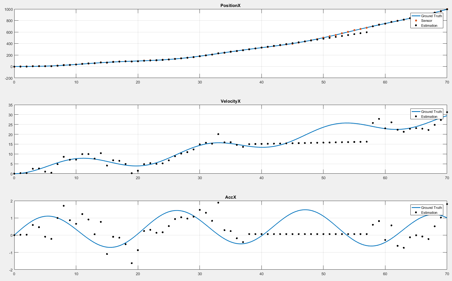
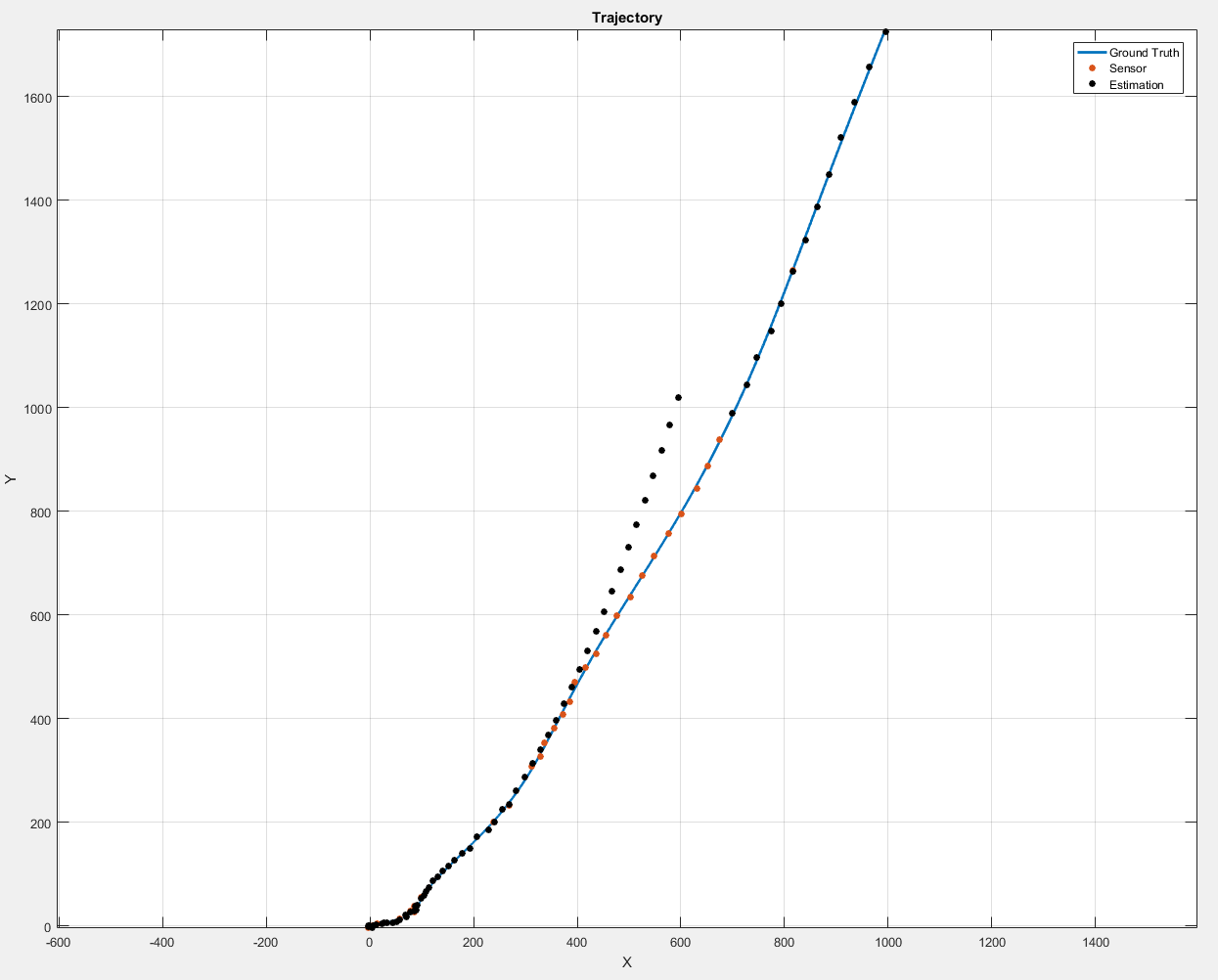
如您所见,即使没有传感器更新,也可以估计位置